Getting Started
The basics
The core of AnisoCADO is centred around the AnalyticalScaoPsf object.
When created it runs a series of setup routines, including creating a PSF
kernel based on the parameters it is passed during the initialisation. This
original PSF kernel is valid for the on-sky coordinate of the natural guide star
(NGS) used to drive the AO correction. It is the “optimal” PSF, and can always
be called up using .psf_on_axis
from anisocado import AnalyticalScaoPsf

psf = AnalyticalScaoPsf(N=512, wavelength=2.15)  # um
kernel = psf.psf_on_axis
The Strehl ratio of this kernel can be found by calling:
psf.strehl_ratio
The quality of the AO correction reduces as one moves away from the guide star.
To sample the PSF at a specific distance from the guide star (i.e. off axis),
use the method shift_off_axis(). AnisoCADO
calculates a new PSF kernel for this coordinate, which is both returned by the
function, and stored internally in .psf_latest
kernel = psf.shift_off_axis(15, -5)   # arcsec
# saved for later under:
kernel = psf.psf_latest
(Source code, png, hires.png, pdf)

The returned kernel object is a numpy array. However AnisoCADO also produces
a FITS HDU object from the psf_latest array when .hdu is called:
image_hdu = psf.hdu
image_hdu is an ImageHDU object, and can therefore
be saved to disk using the standard astropy method .writeto:
image_hdu.writeto("new_scao_psf.fits")
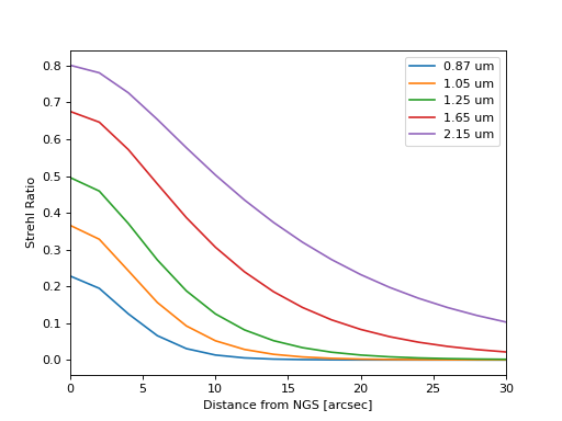
Example: Off-axis Stehl ratios
As an example of using the AnisoCADO API, let’s determine the Strehl ratio for
different wavelengths as we move away from the (on-axis) guide star for the
atmospheric profile EsoMedian
sr_list = {}
wave_list = [0.87, 1.05, 1.25, 1.65, 2.15]
for wave in wave_list:
    sr_list[wave] = []

    # Generate a PSF object for wavelength `wave` in um
    psf = AnalyticalScaoPsf(N=512, wavelength=wave, profile_name="EsoMedian")

    # Shift the PSF to different distances from the NGS
    off_axis_positions = range(0, 41, 2)
    for x in off_axis_positions:
        psf.shift_off_axis(x, 0)
        sr_list[wave] += [psf.strehl_ratio]
(Source code, png, hires.png, pdf)

To plot the results
for wave in wave_list:
    plt.plot(off_axis_positions, sr_list[wave], label="{} um".format(wave))

plt.legend()
plt.xlabel("Distance from NGS [arcsec]")
plt.ylabel("Strehl Ratio")
plt.xlim(0, 30)
(Source code, png, hires.png, pdf)

In-built atmospheric profiles
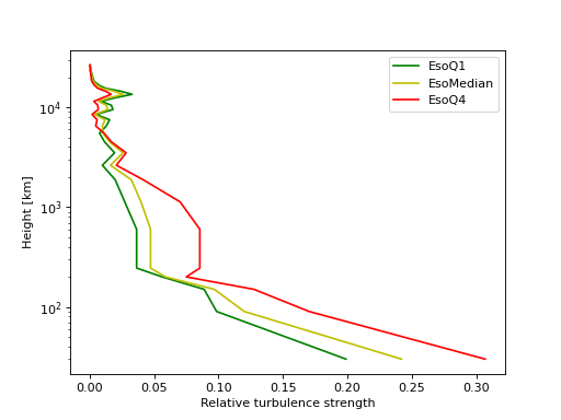
AnisoCADO uses a 35-layer description of the atmospheric turbulence to generate
the PSFs. By default AnisoCADO contains 3 sets of values for the turbulence,
based on the ESO-258292 document. A turbulence profiles can be set by changing
the parameter profile_name of the AnalyticalScaoPsf object:
psf = anisocado.AnalyticalScaoPsf(profile_name="EsoMedian")
# or
psf.profile_name = "EsoMedian"
Alternatively we could set out own atmospheric turbulence profile if we had our own Cn2 information:
psf.layerAltitude = [0.1, 5, 12]    # km
psf.Cn2h = [0.2, 0.5, 0.3]          # relative amount of turbulence
The main 3 atmospheric profiles provided are list in the table below:
Name |
Conditions |
Seeing |
Zenith Distance |
Wind Speed |
Turbulence Profile |
|---|---|---|---|---|---|
EsoQ1 |
Good |
0.4 |
0 |
8.8 |
ESO Quartile 1 |
EsoMedian |
Median |
0.67 |
30 |
10 |
ESO Median |
EsoQ4 |
Bad |
1.0 |
60 |
13 |
ESO Quartile 4 |
(Source code, png, hires.png, pdf)

Creating a field-varying PSF FITS file for SimCADO
AnisoCADO is able to create PSF files in the format needed by SimCADO. The
function anisocado.misc.make_simcado_psf_file handles most of the
nitty-gritty. We just need to provide positions relative to the centre of the
field of view where the PSF should be evaluated, and the wavelength at which
this should be done.
To start the example, let’s create a list of coordinates at 45 degree intervals around concentric circles at increasing radii:
# include the centre of the FOV
coords = [(0, 0)]
radii = [1, 2, 3, 5, 7, 11, 15, 23, 31]
for radius in :
    for ang in np.arange(0, 360, 45):
        coords += [(radius * np.cos(np.deg2rad(ang)),
                    radius * np.sin(np.deg2rad(ang)))]
To make life easier, this code in anisocado.misc:
anisocado.misc.field_positions_for_simcado_psf(radii=radii, theta=45)
Now we just need to decide which wavelengths to add. The function ´make_simcado_psf_file` expects the wavelengths to be in micron [um]. Let’s take the central wavelengths for the 5 major broad-band filters of MICADO:
waves = [0.87, 1.05, 1.25, 1.65, 2.15]
We generate a fits.HDUList object by passing these to list to
make_simcado_psf_file:
from anisocado import misc
hdu = misc.make_simcado_psf_file(coords, waves)
hdu.writeto("my_new_fv_psf.fits")
By default AnisoCADO will create 512 x 512 pixel PSF kernels with a pixel size
of 4mas. If we want to change this we can pass the parameters accepted by
anisocado.psf.AnalyticalScaoPsf as kwargs:
hdu = misc.make_simcado_psf_file(coords, waves, pixelSize=0.0015, N=1024)
Setting atmospheric parameters
A full list of attributes can be found in the docstring for
AnalyticalScaoPsf. The ones most likely to be of interest to the casual
user are given below. They can all be referenced and set in the following
manner:
psf = anisocado.AnalyticalScaoPsf()
psf.profile_name = "EsoQ1"
psf.wavelength = 2.15    # um
Settable Attributes:
profile_name : str
    ['EsoQ1', 'EsoMedian', 'EsoQ4', 'oldEso', 'gendron']. Default: EsoMedian
    Names of specific atmospheric conditions for which presets exist.
    See :func:`psf_utils.get_atmospheric_turbulence`
N : int
    [pixel] Default: 512 pixel. Side-length of the kernel array
wavelength : float
    [um] Default: 2.15 um. Wavelength for which the PSF should be generated
The following parameters can be set by the user, but if they are left blank,
AnisoCADO will fill them in based on the chosen profile_name. As with the
normal attributes, there are many more derived attributes which the user can
override. See AnalyticalScaoPsf.
Derived Attributes if not set by the user:
seeing : float
    [arcsec] Default: 0.67 arcsec. Set by profile_name, if not set by user
zenDist : float
    [degree] Default: 30 deg. Zenith distance. Set by profile_name, if not
    set by user